Note
This technote is a work-in-progress.
1 Abstract
This technote reports the results of three different measurements of AuxTel astigmatism: (1) sweeping a Canon camera through focus (2) sweeping M2 through focus and imaging with LATISS and (3) using the WEP fits to extract Zernike coefficients from the AuxTel donuts. The measured contribution to the seeing from these three techniques is between 0.2 and 0.4 arcsec.
2 Introduction
The SITCom Image Quality team has been tasked with filling out the image quality budget table for AuxTel and determining the main contributions to image degradation in the telescope. Astigmatism is thought to be one of the dominant contributions on AuxTel, and here we quantify it using three different methods and compare the results. We’re also interested in whether there is elevation dependence to the astigmatism.
2.1 Quantifying astigmatism
Astigmatism occurs when two orthogonal axes of a mirror have different radii of curvature, leading to the two axes having different focal lengths. Thus, astigmatism produces an ellipse that is rotated 90 degrees on either side of focus (see Fig. 1). Generally, the best focus for the telescope is halfway between the foci of the two axes, which is where the PSF is circular, not elliptical. The PSF at this location is known as the circle of least confusion.
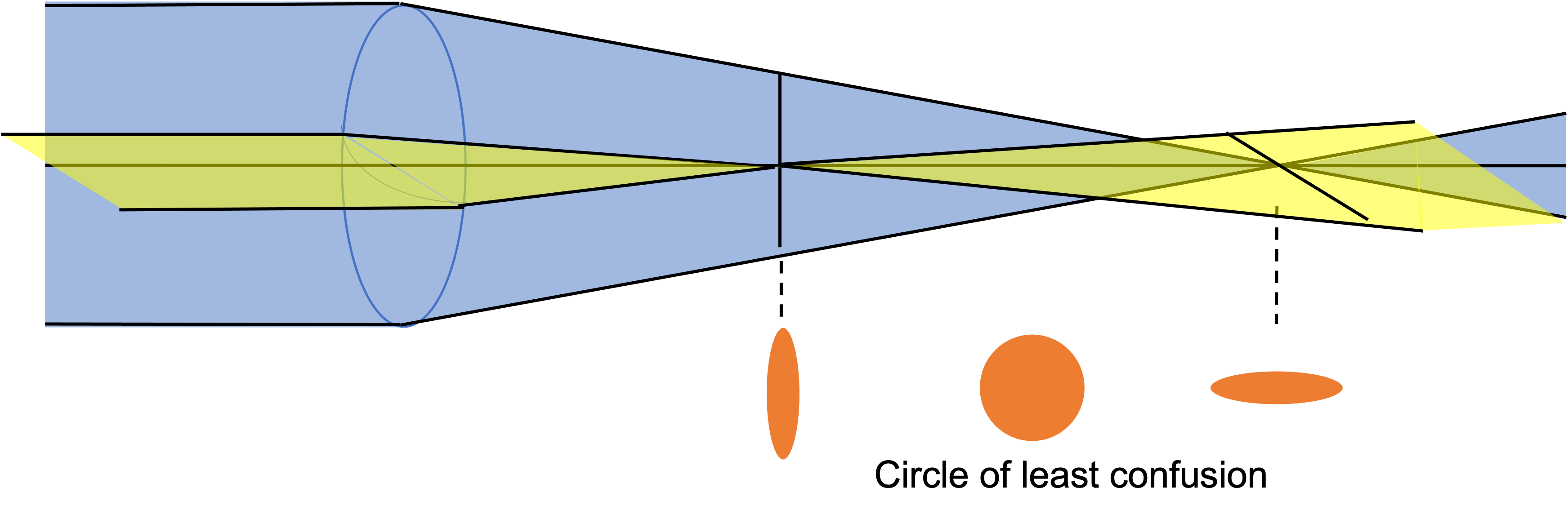
Figure 1 Diagram of astigmatism. Different radii of curvature on the two axes of the lens lead to ellipses on either side of focus.
The first way to estimate the astigmatism is to measure the the distance between the locations of the foci of the two different principle axes of astigmatism. Then the diameter of the circle of least confusion, \(D\), given focal locations \(a\) and \(b\) is:
The other way to compute the astigmatism is to use Zernike coefficients extracted from out of focus donut images.
3 Astigmatism measurements
The three methods we use to compute astigmatism are:
Sweeping a Canon camera to sweep through focus on the second AuxTel nasmyth port.
Sweeping M2 through focus and imaging with LATISS.
Using WEP to extract Zernike coefficients from AuxTel donuts.
3.1 Sweeps through focus with a Canon camera
3.1.1 Method
3.1.1.1 Setup
We performed AuxTel focus tests using a Canon EOS 5D Mark IV without a lens or a color filter. The Canon was mounted on a manually movable stage attached to a rail on the second Nasmyth port. The camera face was flush to the front of the stage (according to wikipedia, the flange focal distance is 44 mm for a Canon EF-mount). The Nasmyth mount ring is 2 cm thick, and there is 1 cm between the mount ring and the optical board, and 7 cm from the start of the optical board to the rail, so for each measurement of stage position on the rail we add 20 mm + 10 mm + 70 mm + 44 mm = 144 mm to report the focus position relative to the output of the AuxTel Nasmyth port.
3.1.1.2 Observations
Images were taken of HD 36787, a magnitude 8 star, from approximately 11:40 pm to 1:20 am local time on Dec. 15-16, 2022 (2:40 am to 4:20 am UTC). The elevation was between 64 and 68 degrees. M2 was first held at its nominal best focus (considered 0 mm for the duration of this note), then moved -1 mm, then moved to +1 mm, then to +0.5 mm, and finally to -0.5 mm. At each M2 position, the camera stage was manually swept through focus in 1mm increments. At each position, four photos with 3.2 s exposure time were taken.
3.1.1.3 Plate scale
For this Canon camera, one pixel is 5.36 \(\mu\) m. Since the aperture of AuxTel is 1.2m and the f-number is 18, the plate scale is \(\frac{5.36e-6 m}{(18 \cdot 1.2m)} \cdot \frac{1}{4.86e-6} = 0.051\) arcsec/pixel.
3.1.2 Results
Images are fit using the GalSim HSM module in python. This method estimates the best-fit elliptical Gaussian to the object. We analyze both the individual images and the coadds of all images taken at the same camera position (simply summing pixels together). Background subtraction is done with 3 \(\sigma\) clipping. See Fig. 2 for background subtracted images swept through focus at M2 = +0.5 mm. The astigmatism was clearly observed at all M2 positions.
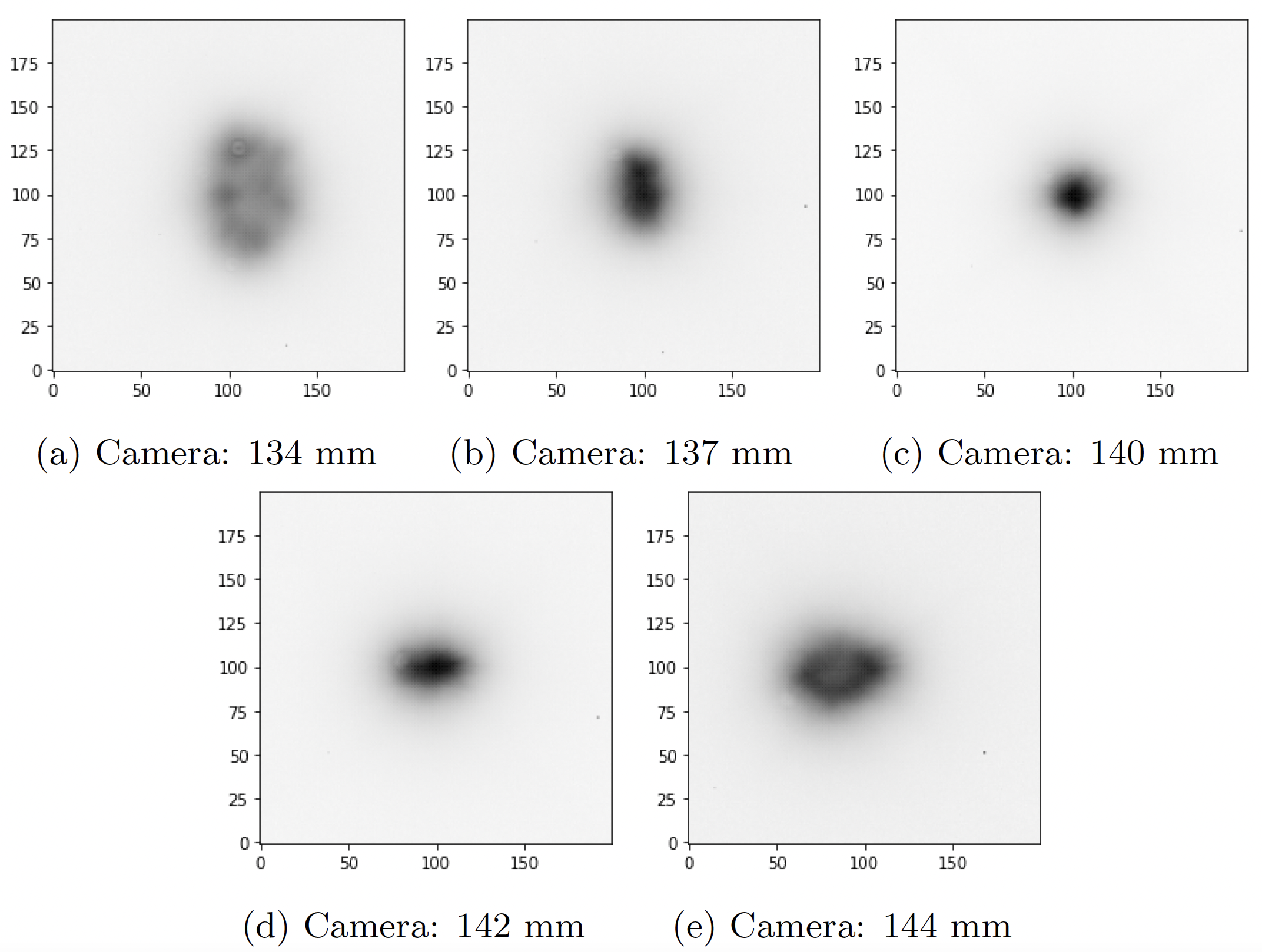
Figure 2 Coadded images from the sweep through focus with the Canon camera where M2 = + 0.5 mm.
3.1.2.1 Focus fits
From GalSim, we get \(\sigma\) for each camera position and M2 position. Shifting the M2 position by 0.5 mm moves the AuxTel focus enough that the camera positions for each M2 position do not overlap (see Fig. 2). Fits are done for each M2 position, using only the individual images where \(sigma < 0.8\) arcsec, to avoid fitting donut images. The fitted minimum \(\sigma\) for each focus position ranges from 0.40 to 0.47 arcsec, with the current optimimum focus at M2 = 0 mm having \(\sigma = 0.43\). However, these datasets were taken over an hour apart, so this is within error for changes in seeing throughout the night. Thus, the M2 position does not seem to be degrading image quality.
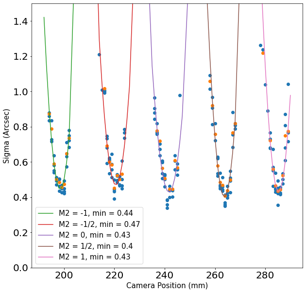
Figure 3 Extracted \(\sigma\) for each camera position. Each parabola corresponds to a different M2 position, from -1 to + 1 mm. Blue points are the extracted \(\sigma\) for individual images. Orange points are the extracted \(\sigma\) for coadded images. Fits are are performed on each M2 position, using only the individual images where \(\sigma < 0.8\) arcsec.
3.1.2.2 Astigmatism measurement
We see clear evidence of astigmatism in the images taken with the Canon camera (see Fig. 2).
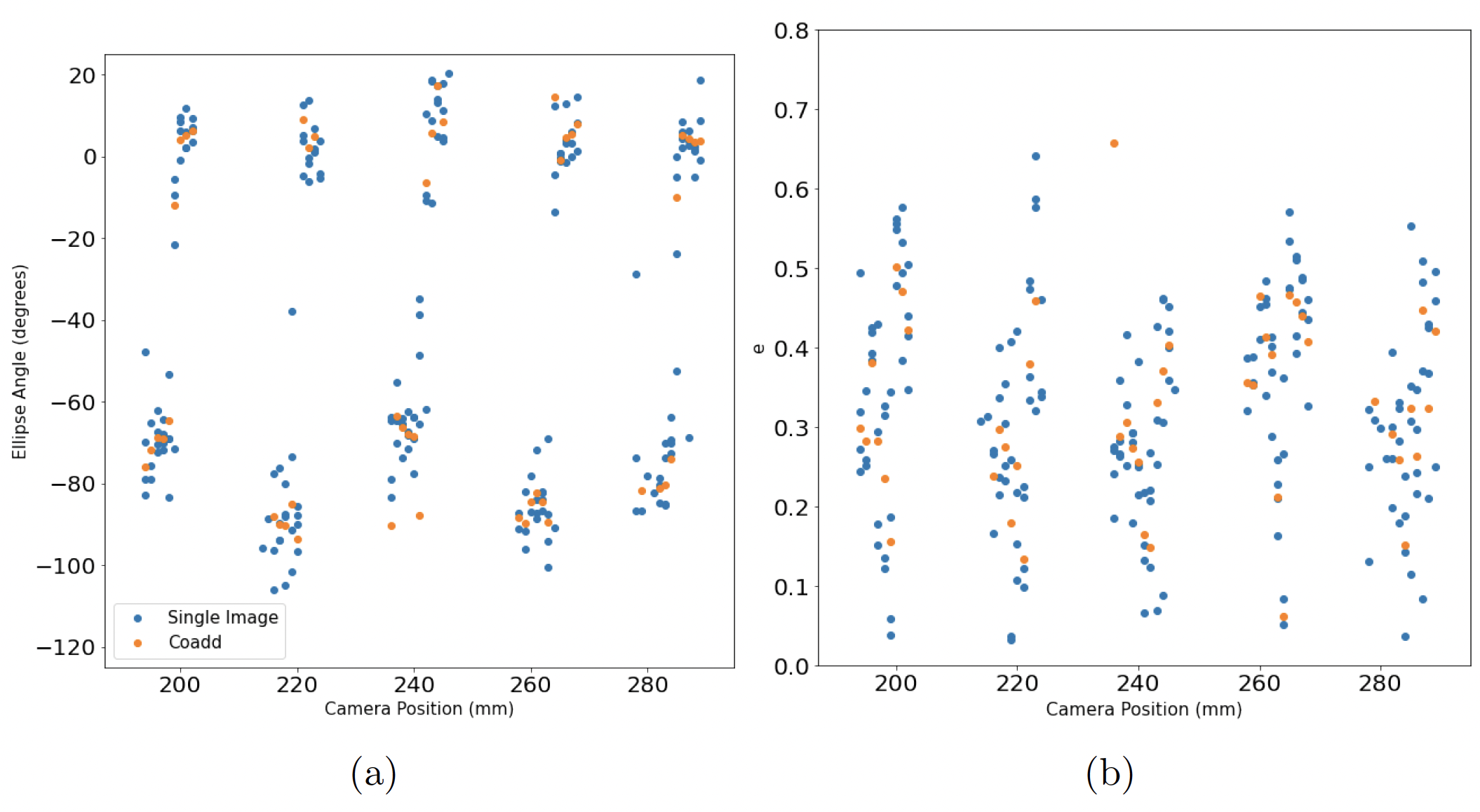
Figure 4 a Extracted ellipse angle for each camera position and b extracted ellipticity \(e\) for each camera position. Blue points are from individual images while orange points are from coadded images.
For a first measurement, we fit a parabola to the minor axis length of each source, as extracted from Galsim (see Fig. 3). We see that the minimum length is 0.05-0.06 arcsec less than the measured \(\sigma\), implying an increased contribution to the FWHM of \(2.35 \cdot \sqrt{0.4^2 - 0.34^2} = 0.5\) arcsec! However, we don’t expect this dataset to be a parabola, but rather a combination of two parabolas, so this may overestimate the seeing due to astigmatism.
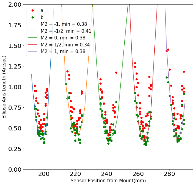
Figure 5 Extracted major and minor ellipse axis for each image at each camera position. Each parabola corresponds to a different M2 position, from -1 to + 1 mm. Red points are the major axis and green points are the minor axis length. Fits are done on the minor axis for each M2 position, using only the individual images where \(\sigma < 0.8\) arcsec.
For a more accurate measurement of astigmatism, we also separate the two axes of the ellipse, \(a\) and \(b\), and fit them individually (see Fig. 4). When we take the average of the best focus values of the two axes and compare to the average value of \(\sigma\), we find an increased contribution to the FWHM of \(2.35 \cdot \sqrt{0.434^2 - 0.415^2} = 0.3\) arcsec.
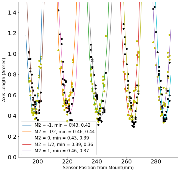
Figure 6 Length of the two orthogonal axes (yellow and black points) of the source. Each pair of parabolas corresponds to a different M2 position, from -1 to + 1 mm. Fits are done using only the individual images where \(\sigma < 0.8\) arcsec.
We also estimate the value of the astigmatism by computing the distance between the minima (or foci) of the two axes, and the diameter, \(D\), of the resulting spot at best focus is given by \(D = 1/f_{number} \cdot (a - b)/2\), which can then be converted to arcsec of seeing. The distance between the foci of the two axes is on average 2.1 mm with a standard deviation of 0.2 mm. This corresponds to a diameter of least confusion of 0.55 \(\pm\) 0.05 arcsec. To determine how this diameter of least confusion contributes to seeing, we convolve a flat top beam with this diameter with a background Gaussian of varying FWHM (see Fig. 5). We see that this corresponds to a seeing of ~0.35 to 0.4 arcsec.
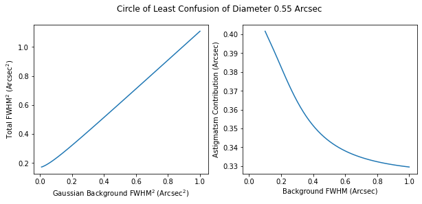
Figure 7 Simulation of contribution to seeing of a beam with a diameter of least confusion of 0.55 arcsec. (a) The total \(FWHM^2\) of the convolution with different background Gaussians and (b) \(\sqrt{Total FHWM^2 - 0.55 arcsec^2}\).
3.2 Sweeps through focus with M2
3.2.1 Method
We sweep M2 through focus from -0.1 mm to 0.1 mm in steps of 0.025 mm, with two 30s exposures taken at each location, then use the same analysis methods as with the Canon camera measurements.
3.2.1.1 Observations
Measurements were taken on 2023-02-14 at around 1:45 TAI with an elevation of 67 degrees and stable seeing conditions. One star selected at random from these images is shown in Fig. 6.
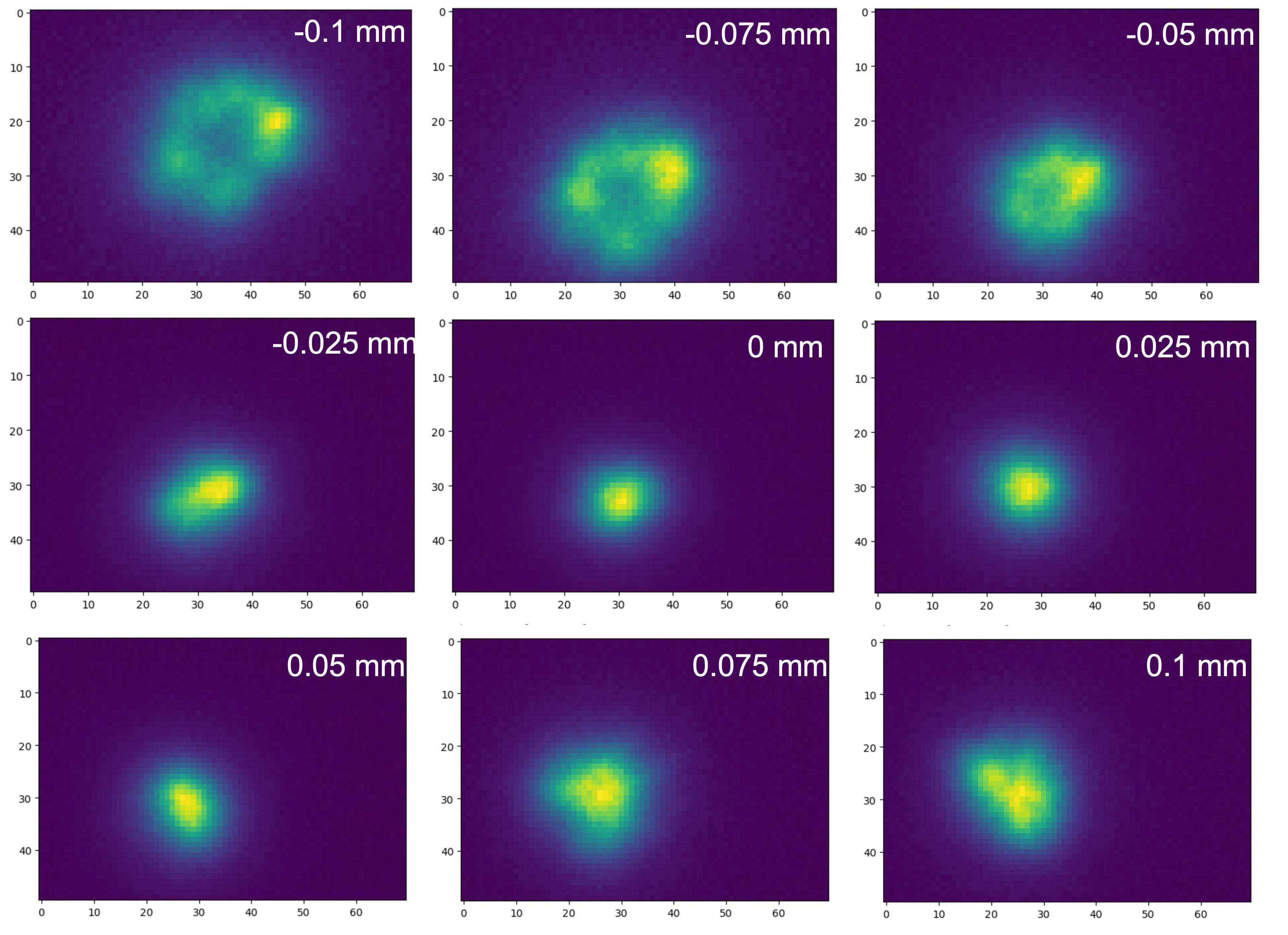
Figure 8 Image of a star from LATISS as M2 is swept through focus. Position of M2 in mm is listed in the top right of each image.
3.2.2 Results
We used the DM singleFrameMeasurementTask package to analyze each frame. The best focus fit is at M2 = 0.026 mm (see Fig. 7), even though WEP was run on the system before taking these measurements.
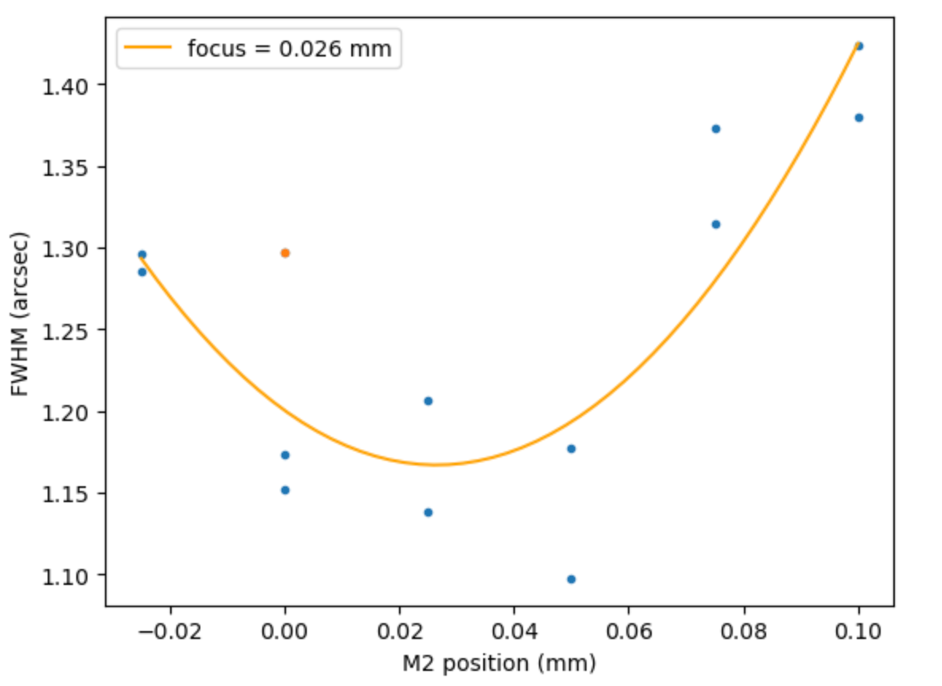
Figure 9 Extracted FWHM vs M2 position for each image taken. Orange dot is first image taken in the sequence, which had a slightly different pointing than the others. It was not used in the fit.
3.2.2.1 Astigmatism measurement
To measure the astigmatism in these images, we diagonalized the Ixx, Iyy, Ixy matrix and took the magnitudes and directions (see Fig. 8) of the eigenvectors.
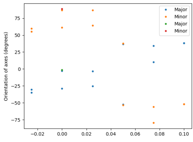
Figure 10 Extracted orientation of the major and minor axis of the PSF for each LATISS image. Orientation came from diagonalizing the Ixx, Iyy, Ixy matrix.
We then took the two axes and fit the eigenvalues of each one separately (see Fig. 9).
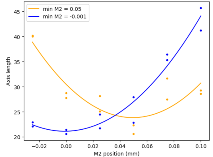
Figure 11 Eigenvalues of the Ixx, Ixy, Iyy matrix. Each axis is fitted separately.
This yields an M2 separation of 0.05 mm between the two foci. This corresponds to \(0.05 \cdot 40 = 2\) mm separation, consistent with what we saw with the Canon camera, corresponding to a circle of least confusion of 0.5 arcsec diameter. This in turn corresponds to a seeing contribution of 0.3 to 0.35 arcsec, depending on the background seeing (see Fig. 9).
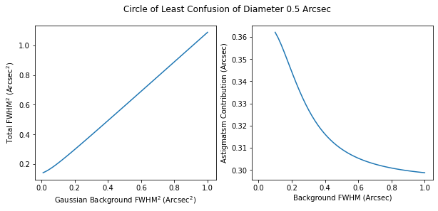
Figure 12 Simulation of contribution to seeing of a beam with a diameter of least confusion of 0.5 arcsec. (a) The total \(FWHM^2\) of the convolution with different background Gaussians and (b) \(sqrt(Total FHWM^2 - 0.5 arcsec^2)\).
3.3 WEP Zernikes
We ran a WEP analysis on all CWFS donut pairs taken on Feb. 16, 2023, which was a night with unusually good atmospheric seeing (the Gemini DIMM reported a seeing of approximately 0.3). To extract the contribution of astigmatism to the seeing, we added the Zernike coefficients (Z5 and Z6 in the Noll convention) in quadrature and multiplied by 1.959. The results can be seen in Fig. 10. There does not seem to be much elevation dependence but there is a range of extracted astigmatism, from 0.1 to 0.3 arcsec, with a clustering at around 0.3 arcsec.
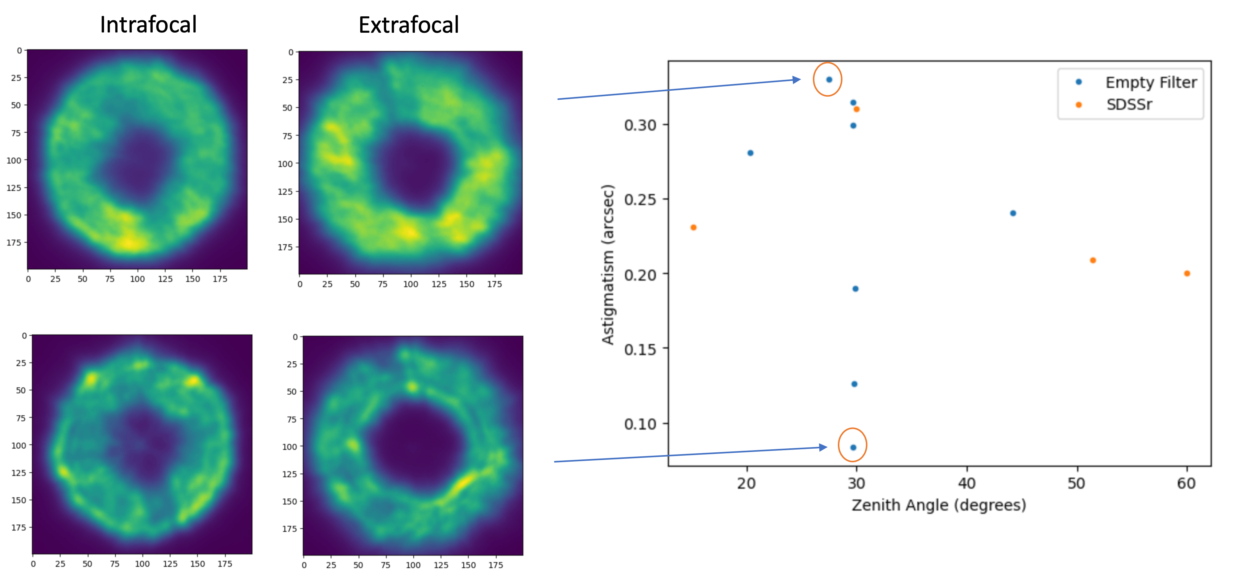
Figure 13 Astigmatism contribution extracted from Zernikes in donut images using WEP.
4 Conclusions and Next Steps
Both of the astigmatism measurements made by sweeping through focus were consistent and imply that astigmatism contributes a seeing of 0.3 to 0.4 arcsec at around 65 degrees. The WEP results are somewhat inconclusive, but seem to imply that the seeing due to astigmatism is between 0.2 and 0.3 arcsec. Regardless, these tests confirm that astigmatism is one of the dominant contributions to the image quality budget for AuxTel.
To more carefully quantify the astigmatism, and understand whether it has an elevation dependence or is caused by M1 or M2, we should run WEP and extract the Zernikes for all old AuxTel datasets and plot astigmatism vs elevation and vs focal plane position. It would also be useful to perform sweeps through focus more frequently, so we can better understand how well the WEP chooses best focus and how long the telescope stays in focus.